Example: 1D Oscillator - Part 3/5

• Author: Dr. Daning Huang

• Date: 07/14/2025

• Updated: 05/07/2026

In this part of the example, we show the setup for data transformations on the input and observation data.

Since Part 2 shows that KBF + weak form is a computationally economic choice, we will stick with this combination in this part.

Preparation

Same drill like in Part 2.

import warnings
warnings.filterwarnings('ignore')
import numpy as np
import torch

from dymad.io import load_model
from dymad.models import KBF
from dymad.training import WeakFormTrainer
from dymad.utils import plot_trajectory, TrajectorySampler

B = 128   # Number of trajectories
N = 501   # Number of steps
t_grid = np.linspace(0, 5, N)

A = np.array([
            [0., 1.],
            [-1., -0.1]])
def f(t, z, u):               # Define the dynamics
    return (z @ A.T) + u
g = lambda t, z, u: z         # Define the observation

# Chirp input for training
config_chr = {
    "control" : {
        "kind": "chirp",
        "params": {
            "t1": 4.0,
            "freq_range": (0.5, 2.0),
            "amp_range": (0.5, 1.0),
            "phase_range": (0.0, 360.0)}}}

# Random Gaussian input for testing/generalization
config_gau = {
    "control" : {
        "kind": "gaussian",
        "params": {
            "mean": 0.5,
            "std":  1.0,
            "t1":   4.0,
            "dt":   0.2,
            "mode": "zoh"}}}

# Generate data
sampler_chr = TrajectorySampler(f, g, config='lti_data.yaml', config_mod=config_chr)
ts, zs, us, xs = sampler_chr.sample(t_grid, batch=B, save='./data/lti.npz')

sampler_gau = TrajectorySampler(f, g, config='lti_data.yaml', config_mod=config_gau)

Set up the options for weak form.

opt_wf = {
    "model": {
      "name" : 'lti_kbf_wf',
      "encoder_layers" : 1,
      "decoder_layers" : 1,
      "hidden_dimension" : 32,
      "koopman_dimension" : 4,
      "const_term" : True,
      "activation" : "none",
      "weight_init" : "xavier_uniform",
      "input_order" : "cubic"
    },
    "criterion": {
        "dynamics" : {"weight" : 1.0},
        "recon" : {"weight" : 1.0}
    },
    "phases" : [{
      "type": "optimizer",
      "name": "WeakForm",
      "trainer": "Weak",
      "n_epochs": 500,
      "save_interval": 10,
      "load_checkpoint": False,
      "learning_rate": 5e-3,
      "decay_rate": 0.999,
      "weak_form_params": {
        "N": 13,
        "dN": 2,
        "ordpol": 2,
        "ordint": 2}
    }]
}

Data Transformation

We will run 3 cases, with transformations specified below:

• No transformation, as in the current lti_model.yaml

• x transforms by standard deviation, u transforms to [0, 1]

• x transforms by standard deviation plus a time delay of 1, u transforms by a time delay of 1

In the last case, a list is used for x to indicate the sequence of transform.

trans1 = {
  "transform_x": {"type": "identity"},
  "transform_u": {"type": "identity"}}

trans2 = {
  "transform_x": {"type": "scaler", "mode": "std"},
  "transform_u": {"type": "scaler", "mode": "01"}}

trans3 = {
  "transform_x": [
    {"type": "scaler", "mode": "std"},
    {"type": "delay", "delay": 1}],
  "transform_u": {"type": "delay", "delay": 1}}

Now Case 1 as a baseline.

The effect of data transformation can be seen in the figure generated on the fly, lti_kbf_wf_prediction.png. Note the range of x and u.

config_path = 'lti_model.yaml'
opt_wf.update(**trans1)
trainer = WeakFormTrainer(config_path, KBF, config_mod=opt_wf)
trainer.train();

Then Case 2. Clearly the ranges of x and u are different.

opt_wf.update(**trans2)
trainer = WeakFormTrainer(config_path, KBF, config_mod=opt_wf)
trainer.train();

Lastly, Case 3. In this case, there are more “states” and “inputs” perceived by the model, due to the time delay.

With time delay, we can also use SDM (Sequential Dynamics Models), that leverage recurrent NN’s. This will be explored in the later part of this example.

opt_wf.update(**trans3)
trainer = WeakFormTrainer(config_path, KBF, config_mod=opt_wf)
trainer.train();

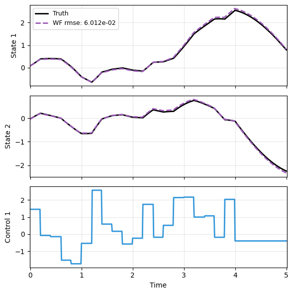
We also show the model prediction for Case 3. The tiny change here is in prd_wf, where t_data is reduced by 1 step, due to the time delay.

The prediction function generated by load_model actually performs a transform and inverse transform on the given x and u, so that one does not need to manually perform the transformation for every new prediction.

ts, xs, us, ys = sampler_gau.sample(t_grid, batch=1, save=None)
x_data = xs[0]
t_data = ts[0]
u_data = us[0]

mdl_wf, prd_wf = load_model(KBF, 'lti_kbf_wf.pt')

with torch.no_grad():
    weak_pred = prd_wf(x_data[:2], t_data[:-1], u=u_data)

plot_trajectory(
    np.array([x_data, weak_pred]), t_data, "LTI",
    us=u_data, labels=['Truth', 'WF'], ifclose=False);