Example: Linear Graph Dynamics - Part 1/2
Author: Dr. Daning Huang
Date: 08/07/2025
Updated: 05/07/2026
Introduction
In the previous examples, we have explored generic dynamical systems, with or without inputs. Here, we take an initial exploration of the graph case.
The dynamical systems on graphs that we consider are of the following:
Think vortices in fluids or electrical devices in power grids, each vortex/device (i.e., nodes) has some states.
The interations are “nearly” local: The rate of change in states at one node is influenced by only the states of neighboring nodes; distant nodes barely have interactions.
To learn this type of dynamics from data, intuitively one would want to exclude terms that are associated with non-existent (distant) interactions. This is where the graph comes in: it tells the model where the interaction exists, so that the model only learns what needs to be learnt.
Using graphs appropriately can be beneficial, including but not limited to: improved accuracy, faster convergence, fewer samples, preserved symmetry, etc.
That said, the goal of this example is to show the API of DyMAD to learn graph dynamics by a graph neural network (GNN). So the example itself will be kept simple - and then one shall see that the procedure is nearly identical to the non-graph cases in the previous examples.
Available Graph Models
In DyMAD, the GNN’s are used in two ways: as autoencoder, and as dynamics.
As autoencoder:
GNN first encodes the states and inputs at each node \((x_i,u_i)\) to latent space \(z_i\), and the latent states per node \(z_i\) are concatenated to produce the full latent states \(z\); in this process, \(z_i\) can depend on the states and inputs from neighboring nodes.
An arbitrary dynamics model can be applied to evolve \(z_i\) - LDM, KBF, Kernel machine, etc., either continuous-time or discrete-time; here, the evolution is independent of other nodes.
Lastly, given new latent states \(z'\), GNN decodes the latent states per node \(z_i'\) to the new states per node \(x_i'\); again, \(x_i'\) can depend on latent states from neighboring nodes.
This type of models are denoted
GXXX, such asGLDMis GNN autoencoder paired withLDMdynamics.
As dynamics:
An arbitrary autoencoder model encodes \((x_i,u_i)\) to latent space \(z_i\); this operation is node-wise and independent of other nodes.
GNN evolves the latent states \(z_i\) per node, and may be impacted (only) by the neighboring nodes.
The autoencoder model decodes new latent states \(z_i'\) to new states \(x_i'\), which again is node-wise and independent of other nodes.
This type of models are denoted
XXXG, such asLDMGis MLP autoencoder paired with GNN dynamics.
In This Example
Part 1 (this page) considers a
GKBFmodel, and apply to an extremely simple example (fixed topology). This is to show the procedure of GNN modeling in DyMAD.Part 2 will consider a
LDMGmodel, and apply to a slightly more complex example with time-varying topologies. This is to illustrate one example where GNN is a natural fit and other methods are inconvenient.
Problem Setup
We will consider the LTI system used before
and concatenate three of the same systems as
There can be two ways to represent this dynamics:
“Naive” approach: Take \(x=[x_1,x_2,x_3]\) and \(u=[u_1,u_2,u_3]\) as distinct features, and learn a generic dynamics \(\dot{x}=f(x,u)\).
Graph approach: Still take \(x\) and \(u\) as features, but learn a node-wise dynamics \(\dot{x}_i=f(x_i,u_i)\), so that \(f\) is shared among the three sets of states.
Next we will take the second approach.
Preparations
As usual the imports. The first cell also normalizes the working directory so the notebook can be launched either from examples/linear_graph or from the repo root without editing paths.
The imports:
from pathlib import Path
import warnings
warnings.filterwarnings('ignore')

import matplotlib.pyplot as plt
import numpy as np
import torch

from dymad.io import load_model
from dymad.models import GKBF, KBF          # G for graph. There are also, e.g., LDM vs GLDM
from dymad.training import WeakFormTrainer  # The use of NODETrainer would be the same
from dymad.utils import TrajectorySampler, adj_to_edge, plot_summary, plot_trajectory

EXAMPLE_DIR = Path.cwd()
DATA_DIR = EXAMPLE_DIR / 'data'
DATA_DIR.mkdir(exist_ok=True)
LTG_DATA_CONFIG = EXAMPLE_DIR / 'ltg_data.yaml'
LTG_KBF_WF_CONFIG = EXAMPLE_DIR / 'ltg_kbf_wf.yaml'
Prepare the data. The LTI system per node:
B = 128
N = 501
t_grid = np.linspace(0, 5, N)

A = np.array([
            [0., 1.],
            [-1., -0.1]])
def f(t, x, u):
    return (x @ A.T) + u
g = lambda t, x, u: x

config_chr = {
    'control': {
        'kind': 'chirp',
        'params': {
            't1': 4.0,
            'freq_range': (0.5, 2.0),
            'amp_range': (0.5, 1.0),
            'phase_range': (0.0, 360.0),
        }}}
A new quantity: adjacency matrix of the graph. This matrix represents the relation among the nodes. The particular choice below assumes equal contributions among the three nodes.
Practically, this is the only new information to be added for GNN modeling.
adj = np.array([
    [0, 1, 1],
    [1, 0, 1],
    [1, 1, 0]
])
Then generate the samples. Since every node is the same, we sample trajectories of one node, and then replicate twice.
sampler = TrajectorySampler(f, g, config=LTG_DATA_CONFIG, config_mod=config_chr)
ts, xs, us, ys = sampler.sample(t_grid, batch=B)
# Pretending a 3-node graph
np.savez_compressed(
    DATA_DIR / 'ltg.npz',
    t=ts, x=np.concatenate([ys, ys, ys], axis=-1), u=np.concatenate([us, us, us], axis=-1),
    adj=adj)
Training
The config file is as follows. The graph-specific option here is gcl under model, which selects the graph convolution layer.
The general entry for training in config is phase. However, when there is only one phase, one can just use training. The WeakFormTrainer still accepts that shorthand and normalizes it into one optimizer phase internally.
"""
data:
  path: './data/ltg.npz'
  n_samples: 128
  n_steps: 501
  double_precision: false

transform_x:
  type: "identity"

transform_u:
  type: "identity"

split:
  train_frac: 0.75

dataloader:
  batch_size: 64

model:
  name: 'ltg_kbf_wf'
  encoder_layers: 1
  decoder_layers: 1
  hidden_dimension: 32
  koopman_dimension: 3
  const_term: true
  autoencoder_type: "cat"
  gcl: "sage"
  activation: "none"
  weight_init: "xavier_uniform"
  input_order: "cubic"

criterion:
  dynamics:
    weight: 1.0
  recon:
    weight: 1.0

training:
  n_epochs: 500
  save_interval: 10
  load_checkpoint: false
  learning_rate: 5e-3
  weak_form_params:
    N: 13
    dN: 2
    ordpol: 2
    ordint: 2
"""
Then the training of graph KBF (GKBF) model. Note it is identical to a regular model training.
config_path = LTG_KBF_WF_CONFIG
trainer = WeakFormTrainer(config_path, GKBF)
trainer.train();
Maybe not surprising, a regular KBF model can be trained using nearly the same setup - we just modify the model name.
But we will not show the results here to keep the example compact.
The graph specific option
gclis ignored in KBF.
"""
config_mod = {
    "model" : {
        "name" : 'ltg_kbf_ng',
        }
}
trainer = WeakFormTrainer(config_path, KBF, config_mod=config_mod)
trainer.train()
"""
Results
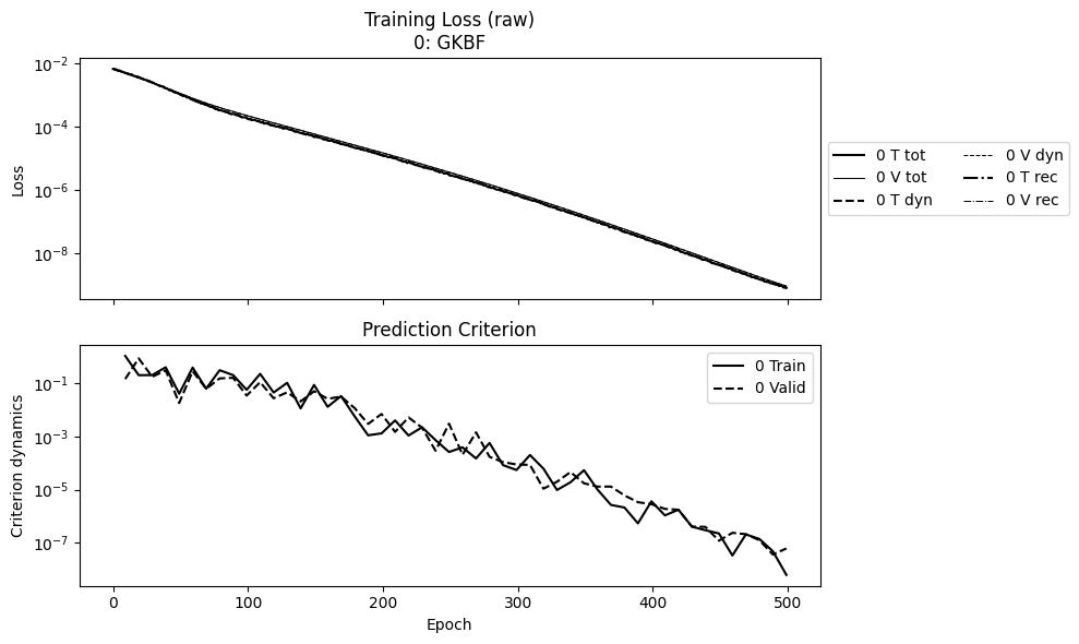
The convergence plots as a rule of thumb:
npz_files = ['ltg_kbf_wf']
npzs = plot_summary(npz_files, labels=['GKBF'], ifscl=False, ifclose=False)
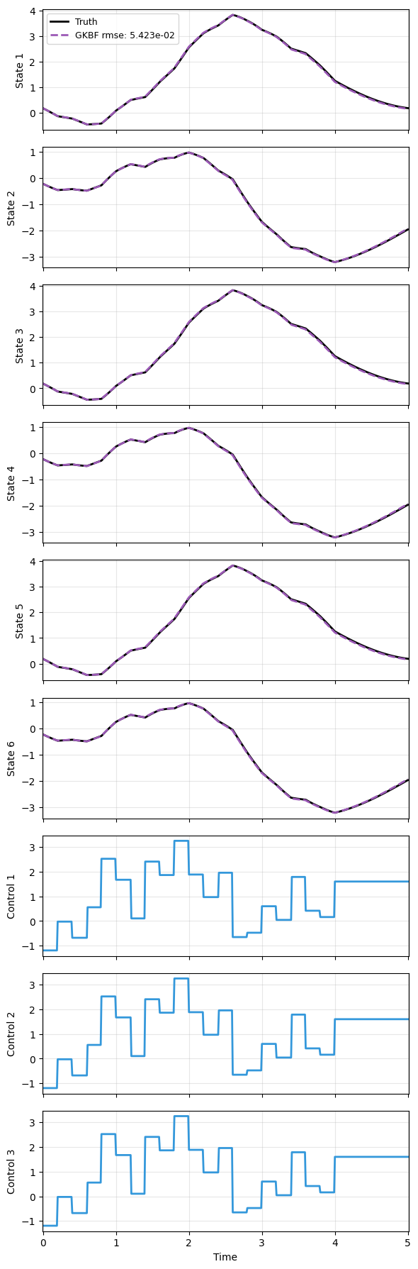
Comparing the prediction, within 200 epochs, GKBF is already able to capture the dynamics fairly well, and more importantly, the three sets of states are identical with the same inputs.
edge_indexis the only new information to be provided.
config_gau = {
    'control': {
        'kind': 'gaussian',
        'params': {
            'mean': 0.5,
            'std':  1.0,
            't1':   4.0,
            'dt':   0.2,
            'mode': 'zoh'}}}
sampler = TrajectorySampler(f, g, config=LTG_DATA_CONFIG, config_mod=config_gau)
edge_index = adj_to_edge(adj)[0]

ts, xs, us, ys = sampler.sample(t_grid, batch=1)
x_data = np.concatenate([ys[0], ys[0], ys[0]], axis=-1)
t_data = ts[0]
u_data = np.concatenate([us[0], us[0], us[0]], axis=-1)

_, prd_g = load_model(GKBF, 'ltg_kbf_wf.pt')

with torch.no_grad():
    g_pred = prd_g(x_data, t_data, u=u_data, ei=edge_index)

plot_trajectory(
    np.array([x_data, g_pred]), t_data, 'LTG',
    us=u_data, labels=['Truth', 'GKBF'], ifclose=False);