Example: Spectral Analysis - Part 1/2

• Author: Dr. Daning Huang

• Date: 09/07/2025

• Updated: 05/07/2026

Introduction

In this example, we explore:

• Part I: The development of models similar to dynamic mode decomposition (DMD)

• Part II: The spectral analysis of such models, including the eigenvalues, eigenmodes, etc.

Specifically, we consider the well-known Van der Pol oscillator,

\[ \ddot{s} - \mu(1-s^2)\dot{s} + s = 0 \]

which exhibits limit cycle oscillation (LCO) for \(\mu>0\).

Basic analysis of the dynamical system would start with rewriting the dynamics in state space form, \(\dot{x} = f(x)\) with \(x=[x,\dot{x}]\), then linearize at the fixed point, and compute the eigenvalues to check stability.

A bit more sophisticated analysis would consider the limit cycle of the system, linearize around this orbit, and find the Floquet exponent to determine the stability of the LCO.

The above two approaches are only valid near the equilibrium (either fixed point or limit cycle). Here what we consider is a Koopman approach, that technically can characterize the dynamics beyond the linearized region (if learned well from data).

In the first part of this example, we show how to learn such models; this is based on functionalities already presented in previous examples, but with a few more tweaks. Then, in the following part, we show how to analyze such models, using another module in DyMAD.

Preparation

As usual, a bunch of imports

import warnings
warnings.filterwarnings('ignore')
import copy
from pathlib import Path

import matplotlib.pyplot as plt
import numpy as np
import scipy.integrate as spi
import torch

from dymad.io import load_model
from dymad.models import DKBF, KBF
from dymad.training import LinearTrainer, StackedTrainer
from dymad.utils import plot_trajectory, TrajectorySampler

Then define the dynamics

SEED = 7
np.random.seed(SEED)
torch.manual_seed(SEED)

B = 500  # Total number of trajectories
N = 81   # Length of trajectory
t_grid = np.linspace(0, 8, N)
dt = t_grid[1] - t_grid[0]

mu = 1.0
def f(t, x):
    _x, _y = x
    dx = np.array([
        _y,
        mu * (1-_x**2)*_y - _x
    ])
    return dx
g = lambda t, x: x  # Observing full states

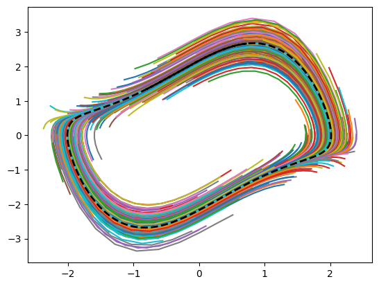
One thing new here is that we would like to sample around the limit cycle, so that the model is more accurate in capturing the characteristics of the LC.

To do so, we first sample a reference trajectory of LC, by running a long simulation and retaining the last portion.

_Nt = 161
_ts = np.linspace(0, 40.0, 8*_Nt)
_res = spi.solve_ivp(f, [0,_ts[-1]], [2,2], t_eval=_ts)
_ref = _res.y[:,-240:].T

Then we use the perturb mode in the sampler, that randomly picks a point in the reference trajectory, and adds perturbation to that point to produce an initial condition. After sampling we plot the trajectories to verify their distributions, where the black dashed line is the reference (i.e., the LC).

"""sa_data.yaml
dims:
  states: 2
  inputs: 0
  observations: 2

solver:
  method: RK45
  rtol: 1.0e-6
  atol: 1.0e-6
"""

db = 0.4
smpl = {'x0': {
    'kind': 'perturb',
    'params': {'bounds': [-db, db], 'ref': _ref}}
    }
sampler = TrajectorySampler(f, g, config='sa_data.yaml', rng=SEED, config_mod=smpl)
ts, xs, ys = sampler.sample(t_grid, batch=B, save='./data/sa.npz')

for i in range(B):
    plt.plot(ys[i, :, 0], ys[i, :, 1])
plt.plot(_ref[:,0], _ref[:,1], 'k--', linewidth=2);

Model Definitions

As usual, start with a YAML file giving the basic configuration,

"""
data:
  path: './data/sa.npz'
  n_samples: 500
  n_steps: 81
  split_seed: 7
  double_precision: true

transform_x:
  type: "scaler"
  mode: "-11"

transform_u:
  type: "identity"

split:
  train_frac: 0.8

dataloader:
  batch_size: 300
"""

We will consider 5 model configurations in this example. The first three are equivalent to the DMD formulation, lifting the states up to 9th order polynomials. The differences are

• No truncation in the least squares step, so the model order is the same as the number of features.

• Standard DMD, that truncates the least squares to rank 15.

• The “ResDMD” approach, that computes a full least squares step, and truncates later by the so-called residual criteria. See, e.g., here

The above 3 configurations share the same model dictionary,

trans = [
        {"type": "scaler", "mode": "-11"},
        {"type": "lift", "fobs": "poly", "Ks": [10, 10]}  # New transformation in pre-processing
    ]
mdl_kl = {
    "name" : 'sa_model',
    "encoder_layers" : 0,         # No autoencoding, since already done by lifting
    "decoder_layers" : 0,
    "koopman_dimension" : 100,
    "activation" : "none",
    "weight_init" : "xavier_uniform",
    "predictor_type" : "exp",}    # Using matrix exponential for prediction, since the whole model is linear

The 3 lifted linear configurations are trained using LinearTrainer. In the current DyMAD API, the linear-solve choice is expressed directly in the training config (method='full', truncated, or sako) rather than through the older nested ls_update block.

SAKO stands for Spectral Analysis of Koopman Operator, where the core algorithms are from ResDMD.

ref = {
    "n_epochs": 1,
    "save_interval": 1,
    "load_checkpoint": False,}
trn_ln = {                        
    "method": "full"}        # No truncation at all
trn_ln.update(ref)
trn_tr = {
    "method": "truncated",    # Truncation to rank 15
    "params": 15}
trn_tr.update(ref)
trn_sa = {
    "method": "sako",         # ResDMD, rank 15
    "params": 15,
    "kwargs": {"remove_one": True}}      # Remove the trivial constant mode
trn_sa.update(ref)

The remaining two model configurations involve autoencoders, assuming a Koopman dimension of 3. One is continuous-time, and the other is discrete-time.

Current DyMAD exposes the mixed linear-solve plus optimizer workflow explicitly through phases, so we use a StackedTrainer schedule that alternates a spectral solve with NODE refinement. In continuous-time, the full_log solve computes the discrete-time matrix first and then takes its matrix log to recover a continuous-time generator. The approach is effective for lower sampling frequencies, but limited to autonomous systems.

mdl_kb = {
    "name" : 'sa_model',
    "encoder_layers" : 2,
    "decoder_layers" : 2,
    "hidden_dimension" : 64,
    "koopman_dimension" : 3,
    "activation" : "prelu",
    "weight_init" : "xavier_uniform",
    "predictor_type" : "exp",}     # Matrix exponential used in the latent space

trn_nd = {
    "n_epochs": 500,
    "save_interval": 100,
    "load_checkpoint": False,
    "learning_rate": 1e-2,
    "decay_rate": 0.999,
}

def _optimizer_phase(cfg):
    phase = copy.deepcopy(cfg)
    phase.update({"type": "optimizer", "trainer": "NODE"})
    return phase


def _linear_solve_phase(method):
    return {"type": "linear_solve", "method": method}


def _spectral_schedule(method):
    return [
        {
            "repeat": {
                "name": "solve_refine",
                "times": 10,
                "phases": [
                    _linear_solve_phase(method),
                    _optimizer_phase(trn_nd),
                ],
            }
        },
        _linear_solve_phase(method),
    ]

Training and Prediction

First train the five configurations

config_path = 'sa_model.yaml'

cfgs = [
    ('dkbf_ln', DKBF, LinearTrainer,   {"model": mdl_kl, "transform_x" : trans, "training" : trn_ln}),
    ('dkbf_tr', DKBF, LinearTrainer,   {"model": mdl_kl, "transform_x" : trans, "training" : trn_tr}),
    ('dkbf_sa', DKBF, LinearTrainer,   {"model": mdl_kl, "transform_x" : trans, "training" : trn_sa}),
    ('kbf_nd',  KBF,  StackedTrainer,  {"model": mdl_kb, "phases" : _spectral_schedule('full_log')}),
    ('dkbf_nd', DKBF, StackedTrainer,  {"model": mdl_kb, "phases" : _spectral_schedule('full')}),
    ]

IDX = [0, 1, 2, 3, 4]
labels = [cfgs[i][0] for i in IDX]

Ignore possible warnings below, that are due to Apple chips.

for i in IDX:
    mdl, MDL, Trainer, opt = cfgs[i]
    opt["model"]["name"] = f"sa_{mdl}"
    trainer = Trainer(config_path, MDL, config_mod=opt)
    trainer.train()

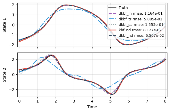
Then predict using one new trajectory to check the performance. The full DMD (dkbf_ln) and the two autoencoder models (dkbf_nd and kbf_nd) perform well. The truncated DMD (dkbf_tr) is far off, while ResDMD (dkbf_sa) is much better at the same rank. A more detailed comparison among the models will be provided in the next part.

sampler = TrajectorySampler(f, g, config='sa_data.yaml', rng=SEED + 1, config_mod=smpl)
ts, xs, ys = sampler.sample(t_grid, batch=1)
x_data = xs[0]
t_data = ts[0]

res = [x_data]
for i in IDX:
    mdl, MDL, _, _ = cfgs[i]
    checkpoint_path = Path(f'sa_{mdl}') / f'sa_{mdl}.pt'
    _, prd_func = load_model(MDL, checkpoint_path)
    with torch.no_grad():
        pred = prd_func(x_data, t_data)
    res.append(pred)

plot_trajectory(np.array(res), t_data, "SA", labels=['Truth'] + labels, ifclose=False);