Example: 2D Koopman - Part 1/3

• Author: Dr. Daning Huang

• Date: 07/28/2025

• Updated: 05/07/2026

Introduction

In the previous 1D Oscillator example, we have covered the basic workflow in DyMAD:

• Generation of data

• Data transformation

• Configuration of model and trainer by YAML and/or dict

• Model training (KBF & LDM with NODE & WF)

• Result visualization

This example explores more features, such as using different autoencoder structures and concatenating two trainers. In addition, here an autonomous system is considered, so that some options can be turned off for simplicity.

Specifically, this time we consider a classical example in Koopman theory,

\[\begin{split} \begin{aligned} \dot{x}_1 &= \mu x_1 \\ \dot{x}_2 &= \lambda (x_2-x_1^2) \end{aligned} \end{split}\]

It is globally stable, and the origin is the equilibrium point.

An interesting fact is that it can be exactly converted to a linear system by introducing a third state \(z_3=x_1^2\):

\[\begin{split} \begin{aligned} \dot{z}_1 &= \mu z_1 \\ \dot{z}_2 &= \lambda (z_2-z_3) \\ \dot{z}_3 &= 2\mu z_3 \end{aligned} \end{split}\]

where \(z_1=x_1\) and \(z_2=x_2\).

Preparation

To start with, the imports:

import warnings
warnings.filterwarnings('ignore')
import matplotlib.pyplot as plt
import numpy as np
import torch

from dymad.io import load_model
from dymad.models import KBF
from dymad.training import NODETrainer, WeakFormTrainer
from dymad.utils import plot_summary, plot_trajectory, TrajectorySampler

B = 256
N = 301
t_grid = np.linspace(0, 6, N)

mu = -0.5
lm = -3
def f(t, x):
    _d = np.array([mu*x[0], lm*(x[1]-x[0]**2)])
    return _d

The options for sampling are collected in kp_data.yaml, which by now should be self-explanatory. Also, the options could be organized as a Python dict too.

"""
dims:
  states: 2
  inputs: 0
  observations: 2

x0:
  kind: uniform
  params:
    bounds:
      - [-2.5, 2.5]
      - [-5.0, 5.0]

solver:
  method: RK45
  rtol: 1.0e-6
  atol: 1.0e-6
"""

Then a two-liner for sampling.

sampler = TrajectorySampler(f, config='kp_data.yaml')
ts, xs, ys = sampler.sample(t_grid, batch=B, save='./data/kp.npz')

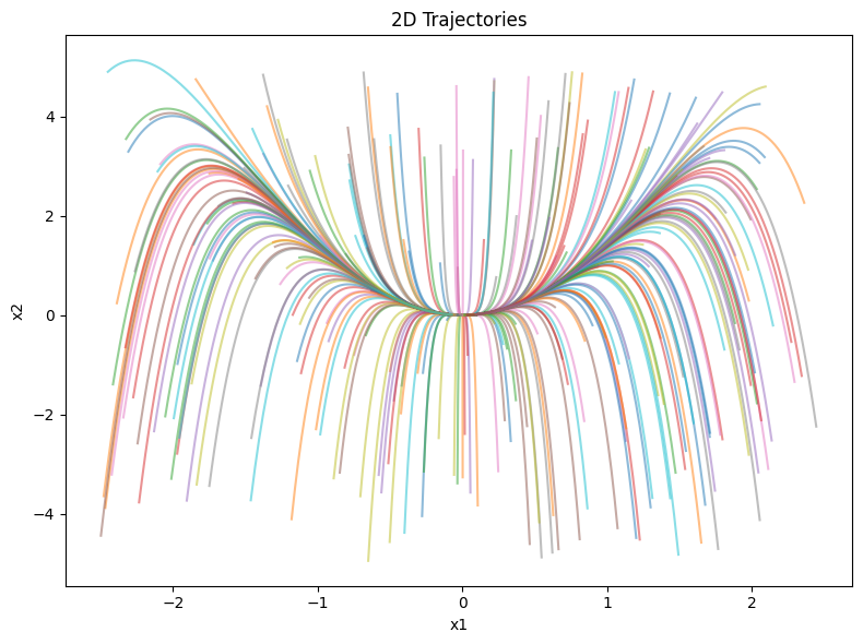
Plotting the trajectories. One can note another feature of the dynamics, that there is a “slow manifold” (the parabolic line, \(x_2-x_1^2=0\)): starting from any point, the states quickly snap to the slow manifold, then slowly move towards the origin.

fig = plt.figure(figsize=(8, 6))
ax = fig.add_subplot(111)
for i in range(B):
    ax.plot(xs[i, :, 0], xs[i, :, 1], alpha=0.5)
ax.set_xlabel('x1')
ax.set_ylabel('x2')
ax.set_title('2D Trajectories')
plt.tight_layout()

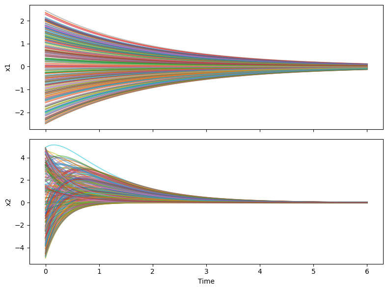
fig, axs = plt.subplots(2, 1, figsize=(8, 6), sharex=True)
for i in range(B):
    axs[0].plot(ts[i], xs[i, :, 0], alpha=0.5)
    axs[1].plot(ts[i], xs[i, :, 1], alpha=0.5)
axs[0].set_ylabel('x1')
axs[1].set_xlabel('Time')
axs[1].set_ylabel('x2')
plt.tight_layout()

Autoencoders

Previously, we used a generic autoencoder,

\[ z = f_{enc}(x),\quad x = f_{dec}(z) \]

which typically requires an additional reconstruction loss during training:

\[ L_{recon} = \sum_i \|f_{dec}(f_{enc}(x_i)) - x_i\|^2 \]

Alternatively, we could use a concatenated structure,

\[ z = [x, \tilde{f}(x)] \equiv f_{enc}(x),\quad x = \text{TakeFirst}(z) \equiv f_{dec}(z) \]

where the output of encoder contains \(x\) and decoder simply takes the \(x\) part as output. The reconstruction loss is 0 by default, which would arguably accelerate the convergence and improve prediction accuracy.

This is a typical technique, e.g., in Koopman learning, although there are limitations on the type of dynamics that it can handle.

Baseline

Next, we first train a KBF model with generic autoencoder as a baseline. To keep the experiment setup readable, kp_model.yaml stores the shared dataset, transform, and base model settings, and the notebook overrides the model, criterion, and training blocks that change between runs.

The shared defaults in kp_model.yaml are:

"""
data:
  path: './data/kp.npz'
  n_samples: 256
  n_steps: 301
  double_precision: true

transform_x:
  type: "scaler"
  mode: "std"

transform_u:
  type: "identity"

split:
  train_frac: 0.75

dataloader:
  batch_size: 256

model:
  name: 'kp_model'
  encoder_layers: 0
  processor_layers: 1
  decoder_layers: 0
  hidden_dimension: 64
  activation: "tanh"
  weight_init: "xavier_uniform"

criterion:
  dynamics:
    weight: 1.0
  recon:
    weight: 1.0
"""

# Options for KBF, generic autoencoder, and weak form
mdl_kb = {
    "encoder_layers" : 2,
    "decoder_layers" : 2,
    "hidden_dimension" : 32,
    "koopman_dimension" : 4,
    "activation" : "prelu",
    "weight_init" : "xavier_uniform"}
crit = {
        "dynamics" : {"weight" : 1.0},
        "recon" : {"weight" : 1.0}}
trn_wf = {
    "n_epochs": 1000,
    "save_interval": 50,
    "load_checkpoint": False,
    "learning_rate": 5e-3,
    "decay_rate": 0.999,
    "weak_form_params": {
        "N": 13,
        "dN": 2,
        "ordpol": 2,
        "ordint": 2}}
mdl_smp = {"name" : "kb_smp"}
mdl_smp.update(**mdl_kb)

config_path = 'kp_model.yaml'

Train the model. We will compare results together with the other case.

trainer = WeakFormTrainer(config_path, KBF, config_mod={"model":mdl_smp, "criterion":crit, "training":trn_wf})
trainer.train();

Variation

Here comes the new autoencoder. This only requires a minimal change: adding an entry autoencoder_type. Here cat points to a predefined autoencoder, that is identity mapping concatenated with a standard MLP.

mdl_cat = {
    "name" : "kb_cat",
    "autoencoder_type" : "cat"}   # New entry
mdl_cat.update(**mdl_kb)

trainer = WeakFormTrainer(config_path, KBF, config_mod={"model":mdl_cat, "criterion":crit, "training":trn_wf})
trainer.train();

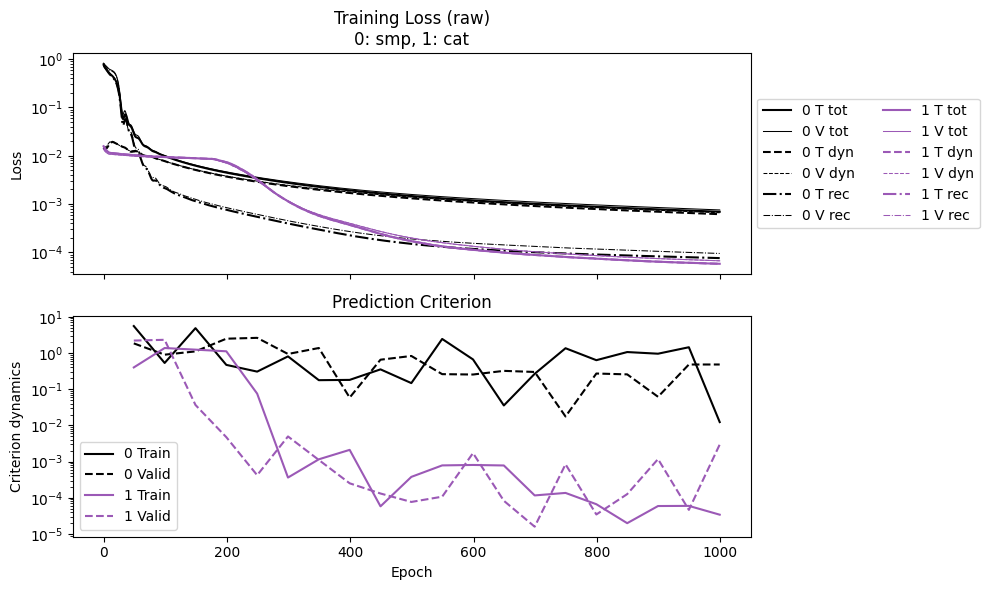
Comparison

Like before, we show two comparisons: convergence history, and prediction on test.

First the convergence. Both results are weak-form, so the losses are comparable. Using the same number of epochs, cat ends up with one-order-of-magnitude lower than smp. The lower loss in cat also brings better trajectory error.

One would also note that in cat, the curve for reconstruction loss is missing. This is because the loss is always zero and thus not shown in log scale.

labels = ['smp', 'cat']
npz_files = [f'kb_{l}' for l in labels]
npzs = plot_summary(npz_files, labels=labels, ifscl=False, ifclose=False)

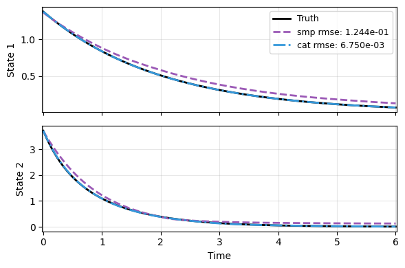
Next, the predictions on a random new trajectory are compared. Clearly, cat beats the generic autoencoder smp.

In the context of Koopman learning, cat is effective for systems with a fixed point, but might not be for others.

ts, xs, ys = sampler.sample(t_grid, batch=1)
x_data = xs[0]
t_data = ts[0]

# The generic case
_, prd_func = load_model(KBF, f'kb_smp.pt')
with torch.no_grad():
    pred_smp = prd_func(x_data, t_data)

# The variation
_, prd_func = load_model(KBF, f'kb_cat.pt')
with torch.no_grad():
    pred_cat = prd_func(x_data, t_data)

# Compare
res = [x_data, pred_smp, pred_cat]
plot_trajectory(
    np.array(res), t_data, "KP",
    labels=['Truth'] + labels, ifclose=False)

array([<Axes: ylabel='State 1'>, <Axes: xlabel='Time', ylabel='State 2'>],
      dtype=object)

Sequential Training

Next, we explore phased training: first optimize the model by weak form for some epochs, then continue with NODE in the same run. The general intuition is the same as before: weak-form training is fast but might not produce highly accurate long-term trajectories, whereas NODE can refine the model once a reasonable warm start is available.

This is a typical continuation strategy in Koopman learning, although there are limitations on the type of dynamics that it can handle.

To do so, we will consider 3 cases for KBF with generic autoencoder:

• Weak form for 1000 epochs

• NODE for 1000 epochs

• Weak form for 500 epochs, then NODE for 500 epochs

Baseline

We have already done the weak-form case. Next let’s complete the NODE case.

mdl_nd = {"name" : "kb_nd"}  # Rename to create a different model
mdl_nd.update(**mdl_kb)

trn_nd = {
    "n_epochs": 1000,
    "save_interval": 20,
    "load_checkpoint": False,
    "learning_rate": 5e-3,
    "decay_rate": 0.999,
    "sweep_lengths": [30, 50, 100, 200, 301],
    "sweep_epoch_step": 200,
    "ode_method": "dopri5",
    "ode_args": {
        "rtol": 1.e-7,
        "atol": 1.e-9
    }
}

trainer = NODETrainer(config_path, KBF, config_mod={"model":mdl_nd, "criterion":crit, "training":trn_nd})
trainer.train();

Sequential Case

The current phased-training API is explicit: each stage is an optimizer phase, and StackedTrainer runs them in order. Here we use 500 weak-form epochs followed by 500 NODE epochs.

from dymad.training import StackedTrainer

mdl_seq = {"name" : "kb_seq"}  # Rename to create a different model
mdl_seq.update(**mdl_kb)
trn_phase = [
    {"type": "optimizer", "trainer": "Weak", **trn_wf},
    {"type": "optimizer", "trainer": "NODE", **trn_nd},
]
trn_phase[0]["n_epochs"] = 500
trn_phase[1]["n_epochs"] = 500

After this, we run the phased trainer.

trainer = StackedTrainer(config_path, KBF, config_mod={"model":mdl_seq, "criterion":crit, "phases":trn_phase})
trainer.train();

Comparison

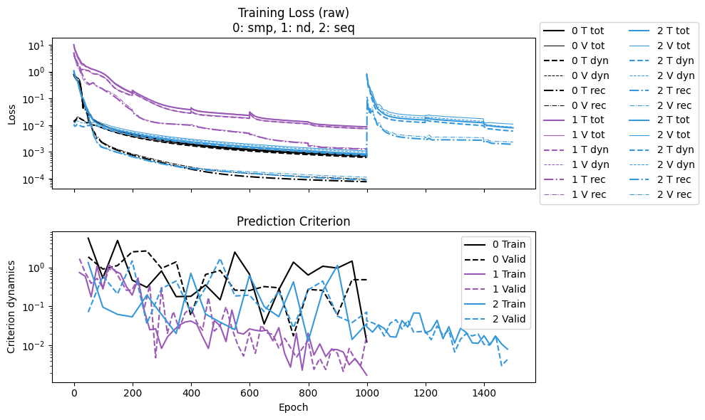
First, the convergence plot. The interpretation of the results should be careful.

• The first segment of seq is comparable to smp, as both are weak-form, and the two do share a similar trend.

• The second segment of seq is comparable to nd, for NODE. Clearly, given a better initial guess, seq starts at a lower loss, and the loss drops much faster than nd.

• Meanwhile, the same prediction criterion is used in both stages, and thus comparable between WeakForm and NODE training. We do see consistent dropping of this criterion as training progresses.

labels = ['smp', 'nd', 'seq']
npz_files = [f'kb_{l}' for l in labels]
npzs = plot_summary(npz_files, labels=labels, ifscl=False, ifclose=False)

print(f"Epoch time wf/nd: {npzs[0]['avg_epoch_time']/npzs[1]['avg_epoch_time']}")
print(f"Epoch time seq/nd: {npzs[2]['avg_epoch_time']/npzs[1]['avg_epoch_time']}")

Epoch time wf/nd: 0.041914277837908506
Epoch time seq/nd: 0.4662447389256852

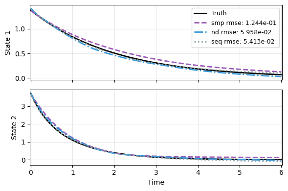
Second, the prediction on test. We recycle the earlier results of smp. nd does improve on smp. But with a bit more cost, seq further improves on nd.

But all of them are worse than cat, highlighting the importance of using the correct structure for learning dynamics.

# NODE
_, prd_func = load_model(KBF, f'kb_nd.pt')
with torch.no_grad():
    pred_nd = prd_func(x_data, t_data)

# Sequential
_, prd_func = load_model(KBF, f'kb_seq.pt')
with torch.no_grad():
    pred_seq = prd_func(x_data, t_data)

# Compare
res = [x_data, pred_smp, pred_nd, pred_seq]
plot_trajectory(
    np.array(res), t_data, "KP",
    labels=['Truth'] + labels, ifclose=False);

For another example of StackedTrainer, see scripts/lti_1s. There, a OneStepTrainer optimizes using a one-step loss and then is used as a warmup phase for NODE.