Example: 2D Koopman - Part 3/3

• Author: Dr. Daning Huang

• Date: 08/15/2025

• Edit: 05/07/2026

As the third part of this example, we show two things:

• A LinearTrainer run that is equivalent to the standard least-squares fitting for a Koopman model.

• The current phased-training workflow for interleaving explicit linear solves with NODE updates.

Preparation

As usual, a few imports:

import warnings
warnings.filterwarnings('ignore')
import matplotlib.pyplot as plt
import numpy as np
import torch

from dymad.io import load_model
from dymad.models import DKBF
from dymad.training import LinearTrainer, NODETrainer, StackedTrainer
from dymad.utils import plot_summary, plot_trajectory, TrajectorySampler

We already have data from Part 1, so no data generation here. The config file kp_model.yaml is the same, too.

As in the earlier parts, kp_model.yaml keeps the shared dataset, transform, and base model defaults, and the cells below override the blocks that change for this section.

Next, the specifications for modeling. We use a concatenation autoencoder, so the reconstruction loss is always zero.

mdl_kb = {
    "name" : 'kp_model',
    "encoder_layers" : 2,
    "decoder_layers" : 2,
    "hidden_dimension" : 32,
    "koopman_dimension" : 8,
    "autoencoder_type": "cat",
    "activation" : "tanh",
    "weight_init" : "xavier_uniform"}

Linear Trainer

The linear trainer only updates the linear part of the model; in the KBF case, this means the system matrices. In this process, the weights in the autoencoder are not updated. The linear components are computed by a least squares problem, standard for Koopman learning:

\[ \min_A \|Z_{n+1}-AZ_n\| \]

where \(Z\) is the collection of encoded states, and \(n\) and \(n+1\) refer to the current and next steps.

The simplest setup is the following. For LinearTrainer, the least-squares choice now lives directly in the training config under method (and optional params). A full solve corresponds to

\[ A=Z_{n+1}Z_n^+ \]

where \(\Box^+\) means pseudo-inverse.

trn_ln1 = {
    "n_epochs": 1,
    "save_interval": 1,
    "load_checkpoint": False,
    "learning_rate": 5e-3,
    "decay_rate": 0.999,
    "method": "full"
    }

We can choose also truncated solution, where params specifies the rank

\[ A=Z_{n+1}V_r\Sigma_r^{-1} U_r^H \]

where \(Z_n\approx U_r\Sigma_rV_r^H\) is an \(r\)th-rank truncated SVD. In the option below, \(r=4\).

trn_ln2 = {
    "n_epochs": 1,
    "save_interval": 1,
    "load_checkpoint": False,
    "learning_rate": 5e-3,
    "decay_rate": 0.999,
    "method": "truncated",
    "params": 4
    }

Next we run the training. The current implementation collects all data samples and performs the least-squares solve once, so each training only needs one iteration.

trn_opts = [trn_ln1, trn_ln2]
config_path = 'kp_model.yaml'

IDX = [0, 1]

for i in IDX:
    opt = {"model": mdl_kb, "training": trn_opts[i]}
    opt["model"]["name"] = f"kp_ln{i+1}"
    trainer = LinearTrainer(config_path, DKBF, config_mod=opt)
    trainer.train()

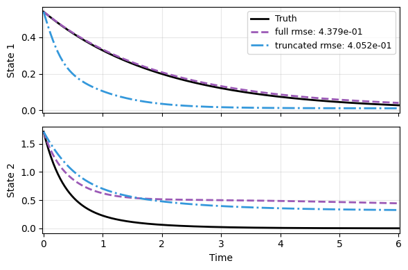
Next, test out the models. Neither of them do well, because the autoencoder is not trained yet. But the least squares do get the model behave roughly like the truth.

N = 301
t_grid = np.linspace(0, 6, N)

mu = -0.5
lm = -3
def f(t, x):
    _d = np.array([mu*x[0], lm*(x[1]-x[0]**2)])
    return _d

sampler = TrajectorySampler(f, config='kp_data.yaml')
ts, xs, ys = sampler.sample(t_grid, batch=1)
x_data = xs[0]
t_data = ts[0]

res = [x_data]
for i in IDX:
    mdl = f"kp_ln{i+1}"
    _, prd_func = load_model(DKBF, f'{mdl}.pt')
    with torch.no_grad():
        pred = prd_func(x_data, t_data)
    res.append(pred)

labels = ['full', 'truncated']
plot_trajectory(
    np.array(res), t_data, "KP",
    labels=['Truth'] + labels, ifclose=False);

Linear-Accelerated Training

The previous results motivate us to take a mixed approach: use explicit linear solves to update the linear part, and let NODE update the full model. This setup is expressed with type: "linear_solve" and type: "optimizer" phases inside StackedTrainer.

trn_ln3 = {
    "n_epochs": 1500,
    "save_interval": 20,
    "load_checkpoint": False,
    "learning_rate": 5e-3,
    "decay_rate": 0.999,
    "sweep_epoch_step": 500,
    "sweep_lengths": [2, 4, 6],
    "chop_mode": "unfold",
    "chop_step": 0.5,
}

The first case below is a pure NODE baseline. The second uses a phased schedule: start with one full least-squares solve, then alternate 100 NODE epochs and another full linear solve for the first 300 epochs, and finish with the remaining NODE epochs.

trn_ln4_chunk = {**trn_ln3, "n_epochs": 100}
trn_ln4_tail = {**trn_ln3, "n_epochs": 1200}
trn_ln4 = [
    {"type": "linear_solve", "method": "full"},
    {
        "repeat": {
            "times": 3,
            "phases": [
                {"type": "optimizer", "trainer": "NODE", **trn_ln4_chunk},
                {"type": "linear_solve", "method": "full"},
            ],
        }
    },
    {"type": "optimizer", "trainer": "NODE", **trn_ln4_tail},
]

The training…

cfgs = [
    ("kp_ln3", NODETrainer, {"model": dict(mdl_kb), "training": trn_ln3}),
    ("kp_ln4", StackedTrainer, {"model": dict(mdl_kb), "phases": trn_ln4}),
]

for name, Trainer, opt in cfgs:
    opt["model"]["name"] = name
    trainer = Trainer(config_path, DKBF, config_mod=opt)
    trainer.train()

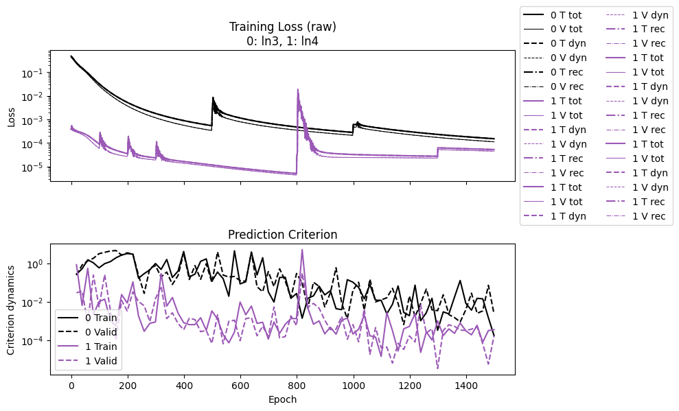
The training would take some time, and here we check the convergence. The definitions of losses are the same, and hence comparable. Clearly the explicit linear-solve phases help with convergence, where the second case starts with a much lower loss and ends lower too.

IDX = [2, 3]
labels = [f"ln{i+1}" for i in IDX]
npz_files = [f'kp_{l}' for l in labels]
npzs = plot_summary(npz_files, labels=labels, ifscl=False, ifclose=False)
for j, i in enumerate(IDX):
    print(f"ln{i+1} Epoch time:", npzs[j]['avg_epoch_time'])

ln3 Epoch time: 0.05018112389246623
ln4 Epoch time: 0.0443859182993571

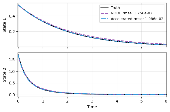
Not surprisingly, the schedule with explicit linear solves produces a much better prediction.

comparison_models = [("kp_ln3", "NODE"), ("kp_ln4", "Accelerated")]
res = [x_data]
for mdl, _ in comparison_models:
    _, prd_func = load_model(DKBF, f'{mdl}.pt')
    with torch.no_grad():
        pred = prd_func(x_data, t_data)
    res.append(pred)

labels = [label for _, label in comparison_models]
plot_trajectory(
    np.array(res), t_data, "KP",
    labels=['Truth'] + labels, ifclose=False);